2 Background

2.1 History

Intravenous fluid therapy first became popular in the cholera epidemic around 1830, when Thomas Latta “threw” several litres of saline into the veins of severely dehydrated cholera patients, and Robert Lewins reported enthusiastically on the “most wonderful and satisfactory effect” [1,2]. However, after the end of the epidemic, the treatment was mostly abandoned. Possibly because the early clinical reports from the epidemic mainly presented temporary effects and mostly in morbidly dehydrated patients, and also because the concerns raised by contemporary sceptics were probably highly relevant—the fluid was both unsterile and unphysiological (hypotonic) [3].

Interest in fluid resuscitation reemerged nearly 50 years later, in 1879, when Kronecker and Sander demonstrated the importance of volume (as opposed to red blood cells) in the treatment of haemorrhage. They bleed down two dogs until bleeding stopped from lack of cardiac activity (approx. 50 % of the blood volume). Then, they reported how resuscitation with an equivalent volume of a saline solution would recover the animals’ cardiac activity [4,5]. This was followed by a number of reports of successful IV fluid resuscitations in humans [5].

Since the end of the nineteenth century, IV fluid administration has been a staple in the treatment of the acutely ill and during surgery. With better equipment and hygiene, the safety of IV fluid administration has increased, and the indication for treatment has widened accordingly—today, IV fluid is even available as a drop-in or home-delivery hangover remedy [6]. Naturally, debates about the appropriate use of IV fluids continue.

2.2 Why give IV fluids?

Fluid should only be administered, when the patient is likely to benefit from it [7]. As a treatment for hypovolemia, the goal is that the infused fluid will increase the circulating volume and thereby the mean systemic filling pressure (see section 2.4.2). This gives an increase in cardiac preload and may, through the Frank-Starling mechanism (see Section 2.4.1), increase CO. This should increase microcirculation and, in turn, the oxygen available to organs, thereby increasing (or retaining) organ function (see Figure 2.1) [8]. As discussed in Section 2.4, this goal is not always achieved.

Figure 2.1: Illustration of the physiological steps from fluid administration to benefit. Reprinted from Monnet et al., 2018 [8] (CC BY).

Another common aim with IV fluid therapy is to resuscitate dehydration, characterised by plasma hypertonicity due to loss of water, e.g., due to gastroenteritis or diabetic polyuria. While hypovolemia can be corrected rapidly with IV infusion of an isotonic fluid, hypertonicity should be corrected slowly through oral intake of water or with IV hypotonic fluid [9]. This dissertation focuses on fluid as a treatment of hypovolemia, and dehydration/hypertonicity will not be discussed further.

During surgery, there is a continuous loss of circulating fluid through urination, bleeding, perspiration and redistribution. If this fluid is not replaced, the patient will gradually become hypovolemic and, eventually, organ failure will occur. Since blood loss and urination is accurately recorded throughout the surgery, the unknown volume of fluid to replace is from perspiration and redistribution [10]. An additional unknown is the patient’s fluid status on arrival to the operating room. Preoperative hypovolemia due to extended fasting before operations used to be a relevant concern, and was treated with significant volumes of fluid during or before induction of anaesthesia [10,11]. With today’s more liberal guidelines for pre-surgery fluid intake, allowing clear fluids until two hours before surgery, the preoperative deficit is probably lower [7,10,12].

With the risk of organ failure from hypovolemia, why not simply give the patient some extra fluid to ensure that there is enough?

2.3 Concerns about liberal use of IV fluids

The statement that IV fluid administration should be treated as any other prescription medication, has become a trope in fluid resuscitation literature [7,13–15]. For good reasons. In addition to the intended effect on CO, summarised in the section above, fluid administration can cause side effects. The principal concerns with excessive fluid administrations can be divided into hypervolemia and non-volume-related effects. The non-volume-related effects depend on the type of fluid. Notable examples include hyperchloremic acidosis from normal saline, and kidney injury associated with hydroxyethyl-starch (HES) infusion [13,16]. Hypervolemia is a more general issue with excessive fluid administration, causing oedemas of tissue and lungs. The pathophysiology of hypervolemia involves both cardiovascular mechanics and endothelial function, so this will be a good place for an introduction to the physiology of fluid administrations.

2.4 The physiology of a fluid bolus

A fluid bolus should increase stroke volume (SV) and, hence, CO. This requires that the fluid remains in circulation to increase cardiac preload, and that this increase in cardiac preload causes an increase in SV. We will start with the latter condition: the Frank-Starling mechanism.

2.4.1 The Frank-Starling mechanism

The relation between cardiac preload and SV is often termed the Frank-Starling mechanism or the Frank-Starling law of the heart, after Otto Frank and Ernest Starling, who are commonly attributed its discovery [17,18]. It has been noted, though, that the phenomenon had been observed several decades earlier [19]. The Frank-Starling mechanism describes that increasing the length of a cardiomyocyte will increase the force generated when the muscle is activated; or, as a consequence, that increased filling of a ventricle will increase stroke volume. The relation occurs only until a certain length or volume, where the curve flattens and the effect eventually reverses. This was clearly demonstrated in experiments by Otto Frank, where he measured the pressure generated through isovolumetric contractions of frog hearts (see Figure 2.2). A number of cellular mechanisms for this length-force relationship has been proposed, but the most important contributors seems to be the following: When cardiac sarcomeres are stretched, the lateral distance between actin and myosin decreases, which increases cross-linking between the filaments and increases Ca⁺⁺ sensitivity. Also, stretching cardiac myocytes increase their Ca⁺⁺ permeability. The drop in force with further stretching has been attributed to a decreasing overlap between filaments, though this mechanism is controversial [20].

Figure 2.2: Otto Frank’s tracings of intraventricular pressure during isovolumetric contractions. In each panel, ventricular volume increases with the number on the tracing. In the right panel, tracing 4 demonstrates the decrease in maximum pressure with overdistension. Reproduction of figures from Frank, 1895 [17], public domain.

A clinical consequence of the Frank-Starling mechanism is that a patient’s SV can only increase from a fluid bolus, if the heart is currently functioning on the rising section of the Frank-Starling curve (see Figure 2.3). A heart’s Frank-Starling curve is, however, not constant, but can be raised with higher sympathetic tone or sympathomimetic drugs (positive inotropes).

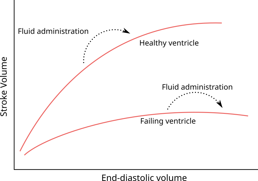
Figure 2.3: Illustration of the Frank-Starling mechanism—the relation between the end-diastolic volume and the stroke volume. If end-diastolic volume is increased in a heart operating on the steep part of the curve (e.g. by a fluid bolus) stroke volume will increase. If the heart is already operating on the flat part of the curve, no increase in stroke volume can be expected.

A few concepts are used interchangeably for both the cause (end-diastolic muscle length) and the effect (contraction) in the Frank-Starling relationship. Starling et al., 1914, note that the physiological relationship must be between the length of a piece of cardiac muscle and the tension it exerts when it contracts, but, since they are not able to measure these in an intact heart, assume that ventricular volume is linearly related to muscle length, and that ventricular pressure is linearly related to muscle tension. They appropriately note that this assumption will become increasingly incorrect with distension and a more globular shape of the ventrice [18]. Other terms used as proxies for end-diastolic muscle length are preload and end-diastolic pressure. Preload should be synonymous with end-diastolic volume or muscle length, but the term is often not well defined. End-diastolic pressure is of course related to muscle length, but it also depends on static mechanical factors (e.g. fibrosis), external pressure and the shape and size of the heart. Proxies for the systolic muscle tension (contraction) include afterload, systolic ventricular pressure, stroke volume and mechanical work (\(pressure \times volume\)).

2.4.2 Venous return and mean systemic filling pressure

Blood circulates from the heart to the arteries, through tissues, to the veins and back to the heart. In steady state, the circulating volume is constant and CO is equal to the venous return to the heart. We can consider a simple model of this system, where blood is pumped from a small elastic compartment into a larger elastic compartment and returned again to the smaller elastic compartment through a tube (see Figure 2.4). The pump is the heart, the large compartment represents the capacitance of venules and veins, and the smaller compartment represents the right atrium and large veins immediately upstream from the heart. Arteries are neglected in this model because of their low compliance relative to the venous system (for an illustration of how the arterial system would fit in this model, see Figure 2.5) [21]. The pressure in the large compartment is the venous pressure (\(P_V\)), the pressure in the smaller compartment is the right atrial pressure (\(P_{RA}\)) and the resistance in the tube is the resistance to venous return (\(R_V\)). If the pump is stopped, both compartments will reach an equilibrium pressure: the mean systemic filling pressure (\(P_{MSF}\)). Often, \(P_V\) is considered equal to \(P_{MSF}\) in this model, since the right atrium and arteries have relatively small volumes, and therefore have little impact on \(P_{MSF}\).

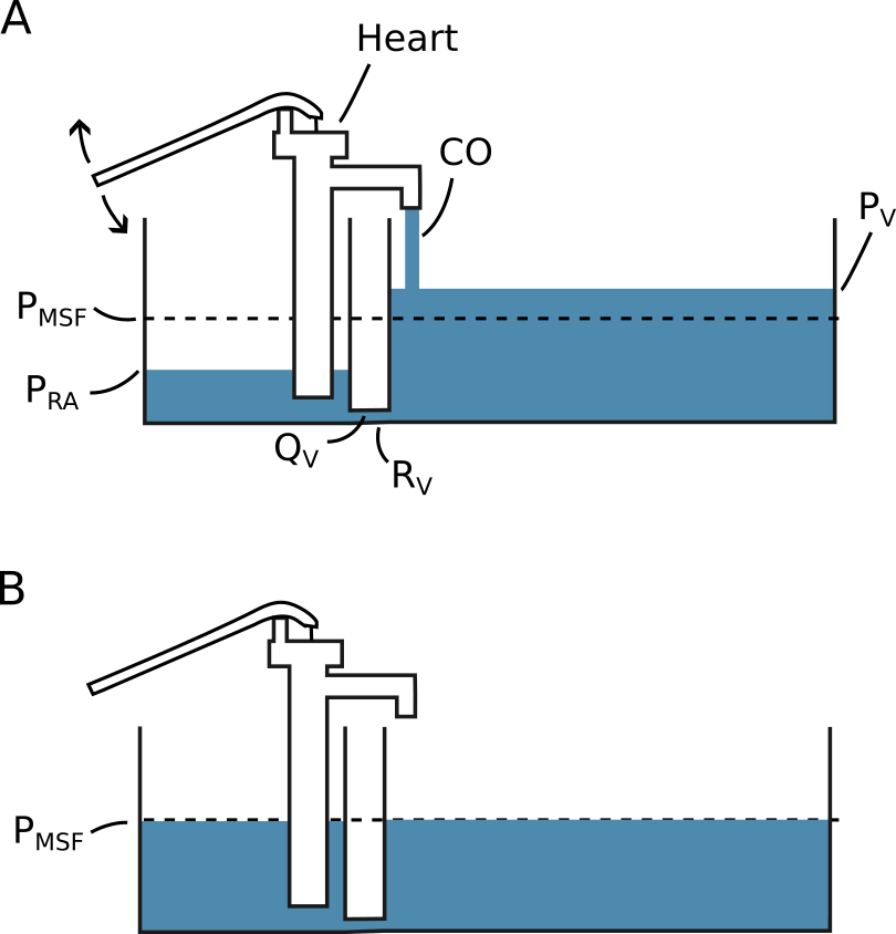
Figure 2.4: A simple model illustrating the concepts of venous return (\(Q_V\)) and mean systemic filling pressure (\(P_{MSF}\)). The pressure is defined by the height of the fluid surface and the compliance is proportional to the width of the compartment. A) The system with a constant cardiac output (CO). B) The system with cardiac arrest (CO = 0). \(P_V\), pressure of the compartment representing venules and veins. \(R_V\), resistance to venous return. \(P_{RA}\), pressure of the compartment representing the right atrium.

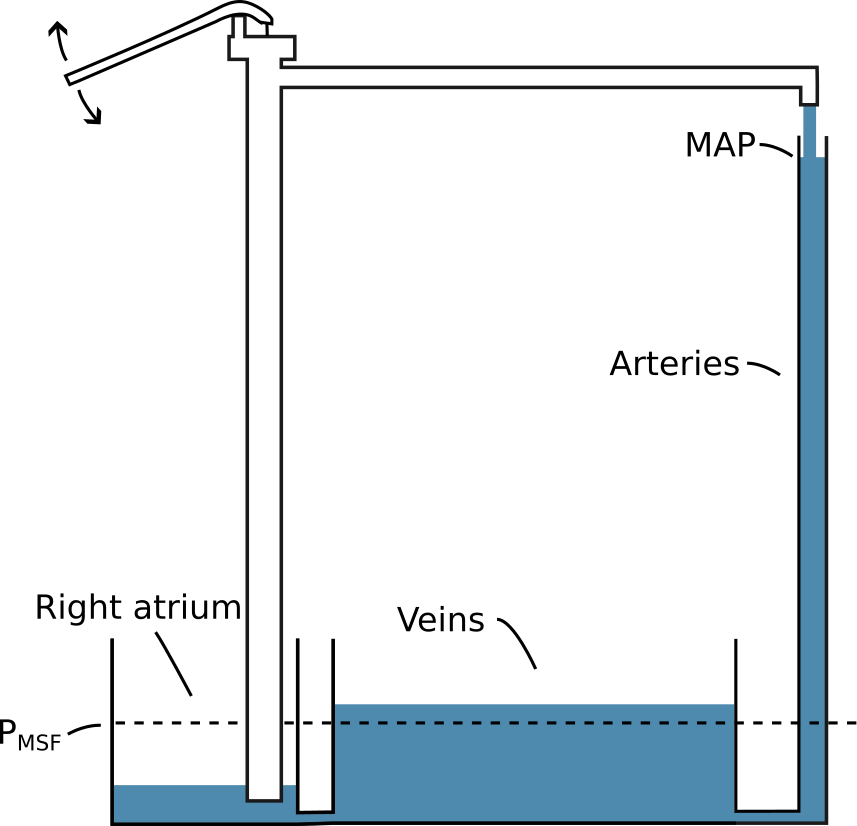
Figure 2.5: An illustration of how the arterial system could be represented in the simple model illustrated in Figure 2.4. MAP, mean arterial pressure.

From this simple model, we can appreciate some factors that determine CO. First, the heart’s ability to pump is an absolute limitation to CO. However, the heart also cannot pump more than what is returned from the veins. This venous return (\(Q_V\)) is determined by the resistance to venous return and the pressure difference between the venous compartment and the right atrial compartment: \[ CO = Q_V = \frac{P_V - P_{RA}}{R_V}. \] Thus, increasing \(P_V\) or lowering \(R_V\) allows a higher CO. If venous compliance is constant, a fluid bolus increases \(P_V\). Alternatively, we can use an \(\alpha\)-adrenergic agonist such as noradrenaline to decrease venous compliance and thereby increase \(P_V\) without adding fluid (venoconstriction will also increase \(R_V\), but the effect on compliance seems to dominate) [22]. Models of venous return often divide compartments into stressed volume and unstressed volume. The unstressed volume is the volume of fluid that will not create any pressure in the compartment—essentially the volume that will remain if the circulation is lacerated. Unstressed volume is effectively inert, and only the stressed volume has any influence on \(Q_V\). Unstressed volume can, however, become stressed through vasoconstriction. While the concept of unstressed volume makes sense anatomically (a vessel can be filled to a certain volume without exerting an elastic recoil), it will often be difficult to differentiate between the effects of unstressed volume becoming stressed and a decrease in compliance of already stressed volume (both increase \(P_{MSF}\)).

As described in the section above, the Frank-Starling curve describes the relationship between ventricular filling and CO (via SV). Ventricular filling is positively related to the \(P_{RA}\), while the \(P_{RA}\) is inversely related to CO, since a high CO will tend to empty the right atrial compartment. The \(P_{RA}\) and CO where \(Q_V\) and CO are in equilibrium can be found as the intersection between the venous return curve (the relationship between venous return and \(P_{RA}\)) and the Frank-Starling curve (a variant with CO rather than SV on the y-axis). This graphical solution, illustrated in Figure 2.6, was first proposed by Arthur Guyton [23].

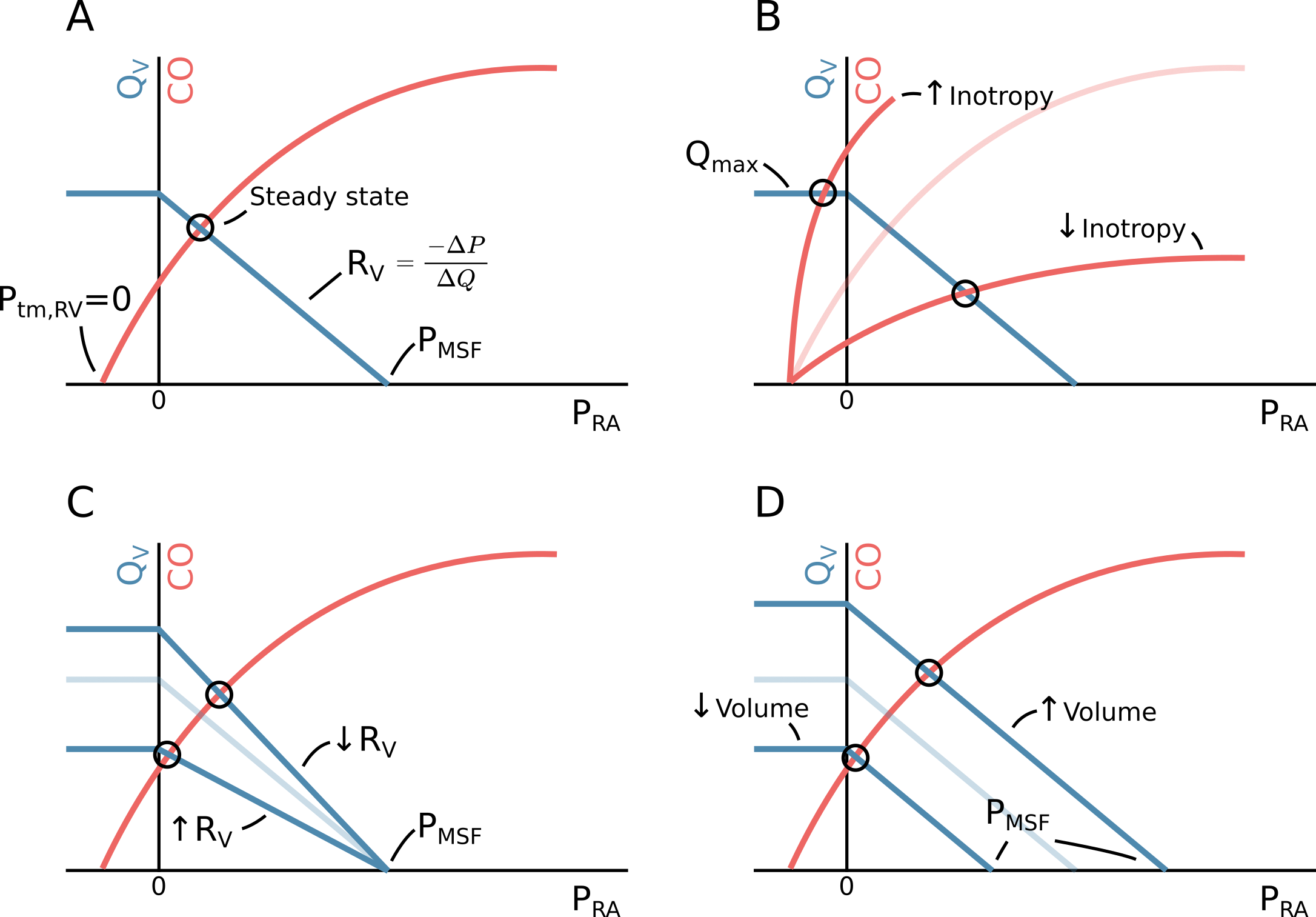
Figure 2.6: A The relationship between venous return (\(Q_V\)), right atrial pressure (\(P_{RA}\)) and cardiac output (CO). If CO (and hence \(Q_V\)) drops to zero, \(P_{RA}\) will equal the mean systemic filling pressure (\(P_{MSF}\)). The circulation is at steady state at the intersection of the venous return function and the cardiac function (when \(Q_V = CO\)). This illustration corresponds to spontaneous breathing, where the intrathoracic pressure is negative. Therefore, the cardiac function starts at a negative pressure where the ventricular transmural pressure (\(P_{tm,RV}\)) is zero. B Change in inotropy or heart rate. C Change in resistance to venous return (\(R_V\)). D Change in \(P_{MSF}\), either via change in stressed volume (fluid bolus) or compliance of capacitance vessels (venoconstriction).

The simple model depicted in Figure 2.4 and Guyton’s graphical solution the steady state CO, provides a basis for understanding clinical interventions that impact CO. One category of interventions target the heart directly by increasing inotropy or chronotropy (increase in cardiac function). A common drug with this effect is dobutamine, which has both positive inotrope and chronotrope effects. In isolation, positive inotropy or chronotropy will increase CO and lower \(P_{RA}\), as depicted in Figure 2.6B. From this figure, we can also identify the theoretical maximum CO obtainable from inotropy or chronotropy: when the heart essentially pumps the right atrium “dry” faster than the venous return can refill it. Since veins are flaccid, they cannot have a transmural pressure below zero. Lowering \(P_{RA}\) below zero (only possible because the intrathoracic pressure is below zero during spontaneous breathing) will not further increase venous return as extrathoracic veins will collapse in proportion to the lower \(P_{RA}\) (depicted as the left steady state point in Figure 2.6B). This is known as the “waterfall effect”, since it is analogous to how changing the lower water level in a waterfall will not affect the flow over the waterfall [24].

A second target for optimising CO, is resistance to venous return (\(R_V\)). This resistance can be greatly increased with liver cirrhosis, and alleviation by transjugular intrahepatic portosystemic shunt (TIPS) increases CO [25]. Late stages of pregnancy can also increase \(R_V\) via compression of the inferior vena cava when the mother is in supine position. Increase in \(R_V\) does not impact \(P_{MSF}\) but reduces \(P_{RA}\) and thereby CO (see Figure 2.6C).

The last point of intervention is \(P_{MSF}\). A fluid bolus will increase \(P_{MSF}\) by increasing stressed volume while maintaining compliance of capacitance veins. Venoconstriction (e.g. with noradrenaline) decreases compliance of capacitance veins, and may additionally mobilise previously unstressed volume. Both effects increase \(P_{MSF}\). An increase of \(P_{MSF}\) increases \(P_{RA}\) (by a smaller amount) and thereby CO on the condition that the heart is operating on the ascending part of the Frank-Starling curve (see Figure 2.6C).

2.4.3 Fluid distribution and oedema formation

A principal adverse effect of fluid administration is oedema: a pathological build-up of fluids in the intercellular tissue or within alveoli. Additional fluid in the interstitium increases the diffusion distance between the capillary blood and the cells, decreasing the rate of oxygen delivery to the mitochondria [26]. Pulmonary oedema has a similar detrimental effect on gas exchange in the alveoli.

The mechanism for oedema formation is classically described with Ernest Starling’s understanding of capillary physiology: The interstitial fluid is in an equilibrium between the colloid-osmotic pressure (oncotic pressure) from the macromolecules in blood and the hydrostatic pressure across the capillary membrane. An increase in stressed volume increases transcapillary pressure, driving fluid into the interstitium until a new equilibrium is reached [27]. Adding to this, crystalloid fluids (e.g. normal saline or acetated Ringer’s solution) dilute plasma, which lowers the oncotic pressure and further promotes the formation of oedema.

In recent years, increasing focus has been on the endothelial glycocalyx layer’s role in fluid resuscitation and oedema formation. The glycocalyx is a gel of macromolecules lining the vascular endothelium [28]. One function of this layer is to form a semipermeable membrane that, in addition to retaining plasma proteins, also retains water to a variable degree. The flow of water from vasculature to tissue may be determined less by oncotic pressure difference and more by the current state of the glycocalyx layer [29]. The permeability of the glycocalyx layer seems to be impacted by volume loading. A proposed mechanism for this regulation is that volume loading increases right atrial pressure, causing release of atrial natriuretic peptide (ANP). ANP increases water filtration and may degrade the glycocalyx [30]. This proposed mechanism has, however, been challenged [31]. Another important cause of glycocalyx degradation is inflammation—especially related to sepsis [32].

2.4.4 How long does a fluid bolus remain in circulation?

Fluids must remain in circulation to improve the patient’s hemodynamic status. Both patient and fluid specific factors impact how long we can expect a fluid bolus to exert its intended effect. The intravascular half-life of a crystalloid infusion is around 20 to 40 minutes in conscious volunteers, while the half-life is more than doubled in surgery with general anaesthesia. Colloids are reported to expand plasma volume with a half-life of two to three hours for both healthy subjects and during surgery (the half-life of the macromolecules themselves in synthetic starches (HES) are much longer than the effect on volume expansion). Generally, a hypovolemic state is associated with a more persistent effect of a volume expansion [33].

2.5 When should fluid be given—and how much?

There are two overall strategies for fluid management: to replace fluids according to a measured or estimated loss or deficit, or to give fluids until a specific hemodynamic target is reached.

The fluid replacement strategy is commonly investigated by comparing a restrictive strategy against a liberal strategy. The terms restrictive and liberal are, of course, relative, and through years with superior results from restrictive fluid regiments, both terms have referred to successively lower volumes. This trend seems to have been concluded with the RELIEF trial [7].

In the RELIEF trial, 3000 patients undergoing abdominal surgery were randomised to either a liberal fluid regimen, expected to give a positive fluid balance, or to a restrictive fluid regimen, expected to give a neutral fluid balance. The liberal group received a median of 6.1 litres of fluid, while the restrictive group received a median of 3.7 litres. There was no difference in disability-free survival between the groups, but the restrictive group had a higher rate of acute kidney injury. The liberal group had a calculated fluid balance of +3.1 litres and gained 1.6 kg weight; the restrictive group had a +1.4 litre fluid balance and gaind 0.3 kg (weight gain was only measured in one third of the patients) [34]. An overall interpretation interpretation has been that a positive fluid balance of 1-2 litres is preferable in major abdominal surgery [35].

The alternative—or complementary—strategy is goal-directed hemodynamic therapy (GDT). Here, patients are treated with fluid, and often vasopressors, to reach a specific hemodynamic target. The aim with GDT is to individualise treatment to ensure that hypovolemic patients get enough fluid, while avoiding fluid overload. A common GDT target is SV optimisation: fluid is given in boluses until SV stops increasing. This is interpreted as the patient’s heart having reached the plateau of the Frank-Starling curve, and that further fluid administration will be futile. An example of GDT was investigated in the OPTIMISE trial [36].

The OPTIMISE trial randomised 724 high-risk, abdominal surgery patients to either SV-guided GDT or usual care. The GDT intervention consisted of a fluid administration algorithm where, first, a patient’s target SV was determined by administering colloid fluid in 250 ml boluses until a new bolus no longer caused a sustained increase in SV above 10%. Afterwards, fluids were administered to maintain this target SV. Additionally, dopexamine (inotrope) was infused at a low rate (0.5 \(\mu\)g kg^-1 min^-1). The study results were inconclusive: they were suggestive of a protective effect of the GDT protocol on adverse events and mortality, though the results were also compatible with there being no difference between groups.

Generally, the effect of GDT is difficult to assess. Both because protocols are numerous and heterogenous and because usual care continues to assimilate the GDT protocols under investigation [7]. A recent systematic review of 76 randomised GDT trials had a conclusion similar to the OPTIMISE trial: GDT might work [37]. The OPTIMISE II trial recently completed inclusion (n = 2502) and will hopefully shed more light on the effects of using a relatively simple SV-optimising protocol [38].

There are some disadvantages to the SV-optimising approach to fluid therapy. First, it requires continuous monitoring of SV or CO. Recent technological advances have broadened the availability of continuous CO monitoring, though the accuracy of these technologies are debated (see Section 3.4.3). Second, it can be argued that if fluid is given until it no longer increases SV, then the last fluid bolus was unnecessary and should not have been given. This could be avoided, if the response to a fluid bolus could be predicted.

2.6 Fluid responsiveness prediction

Fluid responsiveness prediction attempts to answer the question: will this patient benefit from a fluid bolus? More precisely, it attempts to answer whether fluid will increase the patient’s CO, which is a necessary—but not sufficient—condition for benefitting from a fluid bolus (see Figure 2.1).

Clinical observations and measurements have long been used as indications that a patient might benefit from fluid administration. Examples are: tachycardia, hypotension, low central venous pressure (CVP) and high plasma lactate. These clinical findings are all common in hypovolemia, but they also have several other causes. Generally, these findings are poorly related to fluid responsiveness [39–41].

Instead, several dynamic methods for predicting fluid responsiveness have been proposed. Here, dynamic refers to the concept of manipulating the heart’s working position on the Frank-Starling curve, and evaluating the effect on SV (either directly or via a surrogate measure).

2.7 Passive leg raise

The passive leg raise manoeuvre attempts to evaluate the effect of a fluid bolus, without giving any fluid. By raising the patient’s legs, unstressed volume is mobilised, increasing \(P_{MSF}\) analogous to a fluid challenge (see Figure 2.7). If the patient responds to this autotransfusion, they are also expected to respond to a subsequent fluid challenge [42]. Unfortunately, the passive leg raise is rather impractical during surgery.

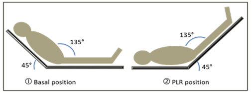
Figure 2.7: Illustration of the passive leg raise (PLR) manoeuvre. From Wikimedia by Patricia.Pineda.Vidal (CC BY)

2.8 The mini-fluid challenge

In the OPTIMISE trial, all fluid challenges were 250 ml, and each bolus was used to determine whether the next bolus should be given. This can be seen as a form of fluid responsiveness prediction: if the patient does not respond to the bolus, there is a low probability that a subsequent bolus will elicit a response; if the patient does respond, the probability is higher, and a subsequent bolus is given (and so on …). If these fluid challenges are used frequently to test fluid responsiveness in a non-responsive patient, it can accumulate to a significant amount of ineffective fluid. A potential solution was proposed by Muller et al. in 2011: the mini-fluid challenge (MFC) [43].

With a MFC, a low volume of fluid, 100 ml, is used to test fluid responsiveness. If the patient responds, 400 ml of fluid is subsequently given. Thus, if a patient is non-responsive to fluid, only 100 ml of ineffective fluid have been given.

The accuracy of the MFC in predicting fluid responsiveness was summarised in a systematic review from 2019 including seven studies [44]. The pooled area under the receiver operating characteristic curve (AUROC) was 0.91, 95% confidence interval (CI) [0.85; 0.97], indicating a highly accurate prediction.

2.8.1 Limitations to the mini-fluid challenge

In most studies investigating the predictive ability of the MFC, SV is measured trice: before the MFC, after the MFC and after the 400 ml bolus. The SV response to the MFC is used to predict the response to the entire 500 ml of fluid given, and the accuracy of this prediction is evaluated. Essentially one change (from 0 ml to 100 ml) is used to predict another change (from 0 ml to 500 ml). Change scores are notoriously difficult to analyse correctly, and most MFC studies do indeed encounter statistical problems. These problems are the topic of Paper 1.

2.9 Pulse pressure variation and heart-lung interaction

Ventilator induced pulse pressure variation (PPV) is the cyclic variation in pulse pressure (PP) caused by mechanical ventilation (see Figure 2.8).

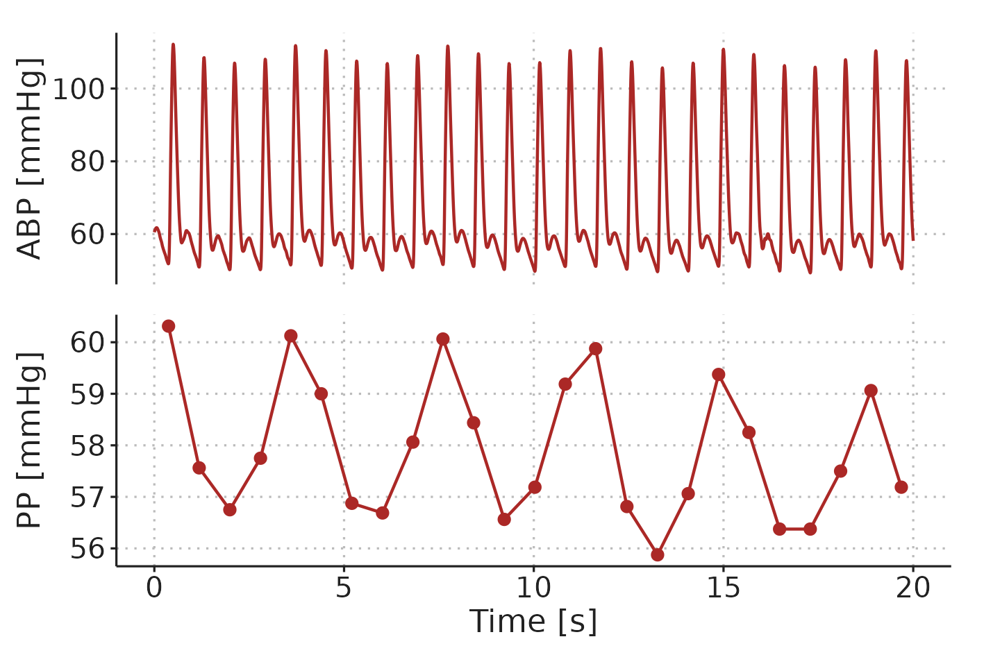
Figure 2.8: Example of ventilator-induced PPV in a patient ventilated with a \(V_T\) of 8 ml kg^-1 and a RR of 17 min^-1. ABP, arterial blood pressure. PP, pulse pressure.

Mechanical ventilation affects circulation in multiple ways [45]. The four principal factors contributing to PPV are illustrated in Figure 2.9. 1) During inspiration, alveolar pressure squeezes out blood from lung capillaries and veins, increasing left-ventricular preload. 2) Lung inflation raises thoracic pressure and aids the flow of blood from the thorax, reducing left-ventricular afterload. Both effects (1 and 2) tend to increase left-ventricular SV during inspiration. Conversely, (3) right-ventricular preload is decreased, since the increased thoracic pressure reduces venous return, and (4) right-ventricular afterload is increased by the alveolar pressure during inspiration. These effects (3 and 4) decrease right-ventricular SV during inspiration. A decrease in right-ventricular SV will decrease left-ventricular preload, but this effect is delayed through the pulmonary circulation. The decreased SV from the right ventricle affects the left ventricle a few seconds later—at the beginning of the expiration—making all four effects contribute to respiratory variation in left-ventricular SV. In most patients, the effect on the right-ventricular preload (3) is the main mediator of ventilator-induced stroke volume variation (SVV) [46].

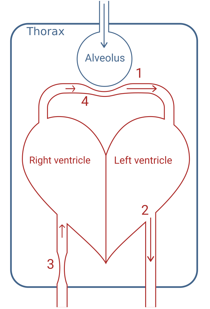
Figure 2.9: Illustration of the three principal effects. 1) Squeeze of peri-alveolar vessels. 2) Higher thoracic pressure facilitates blood flow out of the thorax. 3) Decreased venous return to the right-ventricle due to higher thoracic pressure. 4) Alveolar pressure increases right-ventricular afterload.

Pulse pressure is directly proportional to SV for a given arterial compliance [47]. The cardiac response to the small preload changes caused by the ventilator is therefore reflected in the arterial blood pressure waveform as PPV. Essentially, for a given variation in left-ventricular preload, PPV is proportional to the slope of the Frank-Starling curve at the current preload (see Figure 2.10). Therefore, patients with a high PPV should get an increase in SV if they receive a fluid bolus.

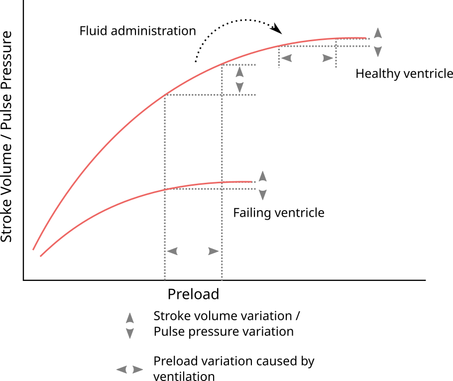
Figure 2.10: Illustration of how PPV reflects the current slope on the Frank-Starling curve, and, therefore, is an indicator of fluid responsiveness.

2.9.1 Pulse pressure variation as a predictor of fluid responsiveness

In the late 1900s, a number of studies found that systolic pressure variation increased with lower circulating volume in both dogs [48,49] and humans [50,51]. In 1998, Tavernier et al. investigated the more clinically relevant question: did high systolic pressure variation predict fluid responsiveness?—it did [52]. The following couple years, results by Michard et al. indicated that PPV was an even better predictor [53,54]. This finding was supported in a systematic review from 2009 that reported a pooled AUROC of 0.94, 95%CI [0.92; 0.96] [55].

2.9.2 Limitations to pulse pressure variation

The use of blood pressure swings induced by heart-lung interactions by mechanical ventilation gained significant interest and scientific credibility in the 1990’s and early 2000’s [56]. In 2005, De Backer et al. published what would become a landmark study regarding limitations to the use of PPV: predicting fluid responsiveness with PPV was less accurate when the \(V_T\) was < 8 ml kg^-1 predicted body weight [41]. This study of 60 patients was soon adopted as firm evidence of the existence of a strict \(V_T\) < 8 ml kg^-1 limitation. The study, however, had some limitations itself. Patients that were ventilated with a low \(V_T\) (< 8 ml kg^-1) also had other unique and possibly confounding characteristics: all but one had acute respiratory distress syndrome (ARDS), while only one had ARDS in the higher \(V_T\) group. Therefore, lung-mechanics, including compliance, were very different between the groups. Respiratory rates were likely also higher in the low \(V_T\) group to maintain adequate ventilation. In later studies the effects of RR and respiratory system compliance was investigated. De Backer et al., 2009 reported that a heart-rate-to-respiratory-rate ratio (HR/RR) < 3.6 markedly reduced PPV [57] (though this effect could also be caused by RR directly), and Monnet et. al. showed in 2012 that low respiratory system compliance (< 30 ml cmH₂O^-1) reduced PPV’s ability to predict fluid responsiveness [58]. Today, all these aspects are considered individual limitations to PPV [56,59]. However, low \(V_T\), high RR and low respiratory compliance often appear together (e.g. in ARDS), and one or more of these circumstances may confounded the others when identifying them as limitations.

Dissecting the effects of \(V_T\) and RR on PPV is the topic of Paper 3, and Paper 2 presents an alternative method for calculating PPV, which may be less sensitive to low HR/RR.

The ventilation-related limitations to PPV presented above are not the only situations where PPV may be unreliable. Some additional limitations are presented here, but these will not be addressed further in this dissertation. The most common limitations to the use of PPV has been summarised with the LIMITS acronym [59]: L is for low HR/RR, which is one of the limitations addressed in this dissertation. I is for irregular heart beats, representing that arrhythmia and frequent extrasystoles causes PPV that is not just related to ventilatory preload variation, but also related to variable intervals between beats. Wyffels et al., 2021 present a promising method for extracting ventilatory PPV in patients with atrial fibrillation, but this method has not yet been clinically validated [60]. M is for mechanical ventilation with \(V_T\) < 8 ml kg^-1: the other limitation addressed in this dissertation. I is for increased abdominal pressure, which primarily refers to laparoscopic surgery. High abdominal pressure decreases thoracic compliance, potentially increasing PPV for a given \(V_T\) [61]. T is for open thorax, where variation in intrathoracic pressure is eliminated. And S is for spontaneous breathing, which also refers to minimally sedated patients whose ventilation is supported by a ventilator. Spontaneous breathing reduces or inverts the ventilatory variation in thoracic pressure, making any resulting PPV difficult to interpret.

2.10 Other dynamic preload indicators

During the past two decades, other dynamic methods for predicting fluid responsiveness have emerged. These include the end-expiratory occlusion test (EEOT) and the tidal volume (\(V_T\)) challenge [62].

Of these, the EEOT is the best validated. The method utilises that an transient end-expiratory occlusion manoeuvre (15 seconds) increases the pressure gradient for venous return (by lowering \(P_{RA}\)), causing a right-shift on the Frank-Starling curve [63]. If the flow response to the EEOT is high, patients are likely to be fluid responders. A systematic review of this method reported an AUROC of 0.96, 95%CI [0.92; 1.00], for predicting fluid responsiveness [44]. The drawback of the EEOT is that it requires active intervention, and patients must be mechanically ventilated with no or little breathing effort. It is best validated with continuous flow monitoring as the predictor, though an increase in PP with end-expiratory occlusion seems to predict fluid responsiveness as well [62]. Also, it may require that the baseline \(V_T\) is >8 ml kg^-1[64]. Most EEOT studies have been conducted in the ICU, and end-expiratory occlusion may not be possible on all anaesthesia machines, potentially limiting the applicability for intraoperative use [65].

The \(V_T\) challenge consists of changing the \(V_T\) from 6 ml kg^-1 to 8 ml kg^-1, causing an increase in PPV [64]. The manoeuvre increases PPV and the increase should be higher in fluid responders. In a recent systematic review that only included a few \(V_T\) challenge studies, the \(V_T\) challenge predicted fluid responsiveness with an AUROC of 0.92 (no CI reported) [66]. The \(V_T\) challenge requires an active intervention, and has the same limitations as PPV itself. When the \(V_T\) challenge is done, and \(V_T\) is 8 ml kg^-1, the \(V_T\) limitation is of course removed. The PPV at a \(V_T\) of 8 ml kg^-1 is in itself predictive of fluid responsiveness, though the \(V_T\) challenge might offer some additional predictive accuracy [64]. However, the performance of the \(V_T\) challenges has rarely been compared to the performance of PPV at \(V_T\)=8 ml kg^-1, and Xu et al., 2022 showed no difference in performance between the two predictors [67].

2.11 Aims

The aim of this PhD was to tackle limitations to two popular methods for fluid responsiveness prediction in the intra-operative setting: PPV and MFC. For PPV, I address the limitations that apply to deeply sedated patients in sinus rhythm undergoing open, non-thoracic surgery.

The aim of Paper 1 was to explain a statistical problem with the design used in most studies of the MFC’s ability to predict fluid responsiveness, and to propose a better design.

The aim of Paper 2 was to introduce generalized additive models (GAMs) as a tool for analysing medical time series and waveforms, to propose how PPV derived from a GAM could help overcome the low HR/RR limitation, and to propose more advanced and experimental use cases of GAMs.

The aim of Paper 3 was to analyse the effects of \(V_T\) and RR on PPV, and to investigate how these ventilator settings impacted PPV’s ability to predict fluid responsiveness.